Introduction & Theory
| Tutorial | |
|---|---|
| Title: | Benchmarking & Scaling |
| Provider: | HPC.NRW
|
| Contact: | tutorials@hpc.nrw |
| Type: | Online |
| Topic Area: | Performance Analysis |
| License: | CC-BY-SA |
| Syllabus
| |
| 1. Introduction & Theory | |
| 2. Interactive Manual Benchmarking | |
| 3. Automated Benchmarking using a Job Script | |
| 4. Automated Benchmarking using JUBE | |
| 5. Plotting & Interpreting Results | |
Scalability
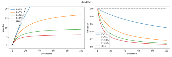
Often users who start running applications on an HPC system tend to assume the more resources (compute nodes / cores) they use, the faster their code will run (i.e. they expect a linear behaviour). Unfortunately this is not the case for the majority of applications. How fast a program runs with different amounts of resources is referred to as scalability. For parallel programs a limiting factor is defined by Amdahl's law. It takes into account the fact, that a certain amount of work of your code is done in parallel but the speedup is ultimately limited by the sequential part of the program.
Strong Scaling
Amdahl's Law
We assume that the total execution time of a program is comprised of
- , a part of the code which can only run in serial
- , a part of the code which can be parallelized
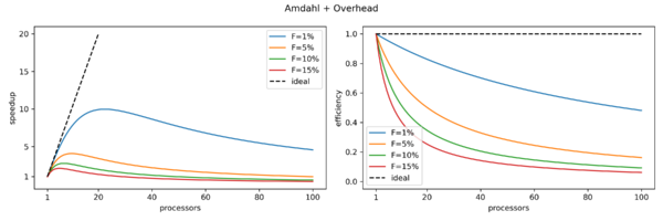
- , parallel overheads due to, e.g. communication
The execution time of a serial code would then be
The time for a parallel code, where the work would be perfectly divided by processors, would be given by
is the speed up amount of time due to the usage of multiple CPUs. The total speedup is defined as the ratio of the sequential to the parallel runtime:
The efficiency is the speedup per processor, i.e.
Speedup and Efficiency
Knowing that , and writing as the fraction of the serial code, we can rewrite this to
This places an upper limit on the strong scalability i.e. how quickly can we solve a problem of fixed size by increasing . It is known as Amdahl's Law.
Consequences
- The speedup is never linear in P, therefore the efficiency is never 100%
- Examples:
- For P=2 processors, to achieve E=0.9, you have to parallelize 89% of the code
- For P=10 processors, to achieve E=0.9, you have to parallelize 99% of the code
- For P=10 processors, to achieve E=0.5, you have to parallelize 89% of the code
Weak Scaling
Fortunately for us, the amount of resources scale well with the problem size. Therefore, instead of throwing large amounts of resources at small problem sizes, we can instead try to increase our problem size as we increase the amount of resources. This is referred to as weak scaling.
Gustafson's Law
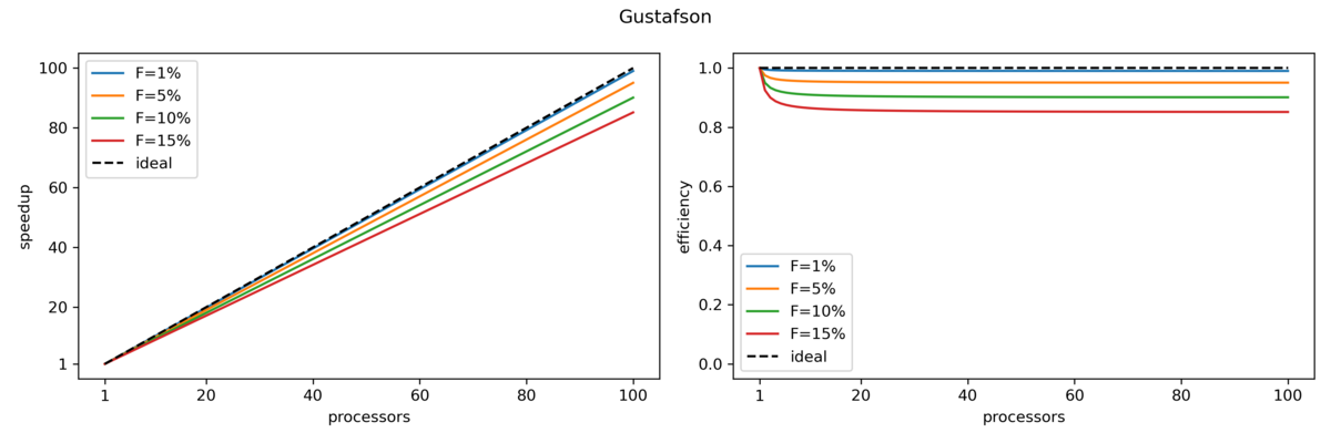
Gustofson's law states that the parallel part of a program scales linearly with the amount of resources while at the same time the serial part does not increase with increasing problem size. The speedup is here given by
where P is the number of processes, F is again the fraction of the serial part of the code and therefore (1-F) the fraction of the parallel part.
With Gustafson’s law the scaled speedup increases linearly with respect to the number of processors (with a slope smaller than one), and there is no upper limit for the scaled speedup. This is called weak scaling, where the scaled speedup is calculated based on the amount of work done for a scaled problem size (in contrast to Amdahl’s law which focuses on fixed problem size). If we apply Gustafson’s law to the previous example of s = 0.05 and p = 0.95, the scaled speedup will become infinity when infinitely many processors are used. Realistically, if we have N = 1000, the scaled speedup will be 950.
Speedup and Efficiency
Consequences
Knowing about speedup and efficiency we can now try to measure this ourselves.
Next: Interactive Manual Benchmarking
Previous: Overview


